$\LaTeX$ 札记（六）——MATLAB与TikZ绘图

在跨年前夜水一片博客，2023年没怎么写博客，因为没有什么可写的~ 祝大家新年快乐哦！

这篇札记主要分为以下几个方面：

如何将MATLAB画的图导出为 $\LaTeX$ 中画图的Ti $k$ Z代码
如何在 $\LaTeX$ 中画图代码进行一些修饰和改进
如何将论文中所有采用Ti $k$ Z的绘图保存为PDF图片，方便后续交稿等操作

首先回答一个问题——“为什么想要把MATLAB画好的图多此一举地转为TikZ？”

TikZ是MATLAB比较原生的绘图方式，所以画图的字体什么的会比较贴近于正文，同时不同图片大小也方便统一。
如果我们需要增加/删减图片的某条线，修改图片某个图例等。
- 如果采用MATLAB导出的方式，工作流是“修改MATLAB画图代码=>导出PDF/EPS=>删减白边=>重新复制到LaTeX文档目录下”；
- 然而如果采用TikZ的方式，我们只需要在第一次复制到相应的文档目录，调整好尺寸大小，后续的几乎所有操作都可以在LaTeX编辑器中完成，而不需要再大费周折从MATLAB导出。

导出MATLAB绘图至TikZ

这里要使用一个MATLAB脚本matlab2tikz：下载链接🔗GitHub - matlab2tikz/matlab2tikz: This program converts MATLAB®/Octave figures to TikZ/pgfplots figures for smooth integration into LaTeX.

首先按照网站Installation部分的安装matlab2tikz
- 把它完整下载到本地。
- 下载完成后，将下载获得的文件夹中的\src文件夹添加到matlab路径中。如addpath('你的目录\src')
在你所需绘图的图片下方输入该命令
1
matlab2tikz('ABCDE.tex');
或者（不显示一长串的说明）
1
matlab2tikz('plot_rebuttal/ABCDE.tex','showInfo',false)
于是你会在你的当前目录下，或者对应文件夹下找到生成的ABCDE.tex文件，这个文件就是tikz的画图函数。主要包含以下一些
- 颜色的定义\definecolor
- \begin{tikzpicture} tikz画图环境
- \begin{axis} axis坐标环境：在axis环境中主要包括坐标区域和legend的定义，以及各个线条的坐标数值。

将这个放置到latex项目的对应路径下，即可在论文中引用它。

注意在最开始的导言区需要引用以下宏包和指令，大家也可以直接粘贴上述生成.tex文档时matlab中的输出：

\usepackage{pgfplots}
\pgfplotsset{compat=newest}
%% the following commands are needed for some MATLAB2tikz features
\usetikzlibrary{plotmarks}
\usetikzlibrary{arrows.meta}
\usepgfplotslibrary{patchplots}

与普通图片相同的是——我们同样需要在figure环境中引用他
与普通图片不同的是——我们不再采用类似\includegraphics[width=.9\linewidth]{img/BCDEF.pdf}的形式来引用图片，而利用类似文件嵌套的形式\input{img/ABCDE}来引用图片，注意到这里我们不需要加入后缀.tex。注意到这里我们不能加入对于大小的控制，对于大小的控制我们会在第二节中阐述。

给出两个例子：
①全图形式：和普通的图片类似，只是\includegraphics变为\input

\begin{figure}[htbp]
    \centering
    \input{main/chapter4/figures/AAAA}
    \caption{OFDM-AAAA}
    \label{fig:postion}
\end{figure}

②子图形式（figure*是IEEEtran格式定义的环境，大家用普通的figure环境即可，\subfloat需要引用subcaption宏包；此外大家也可以直接把子图的注释直接写在[]中）

\begin{figure*}[t]
    \subfloat[]{\input{img/3a_throughput}\label{fig:aaa}}\hfill
    \subfloat[]{\input{img/3b}\label{fig:bbb}}\hfill
    \subfloat[]{\input{img/3c}\label{fig:ccc}}\hfill
    \subfloat[]{\input{img/3d_new}\label{fig:ddd}}
    \caption{(a) xxxxxx. (b) xxxxxx. (c) xxxxxx. (d) xxxxxx. }
    \label{fig:xxxx}
\end{figure*}

【附】如果我们自己用tikz画的图则直接包裹在figure和tikzpicture环境中即可，不需要另开一个文件也可以。将画图单独提取为一个文件主要为了论文中结构清晰。

在LaTeX中修饰TikZ的绘图

本节中我们的操作均对于matlab2tikz生成的.tex操作！

常规操作

大小

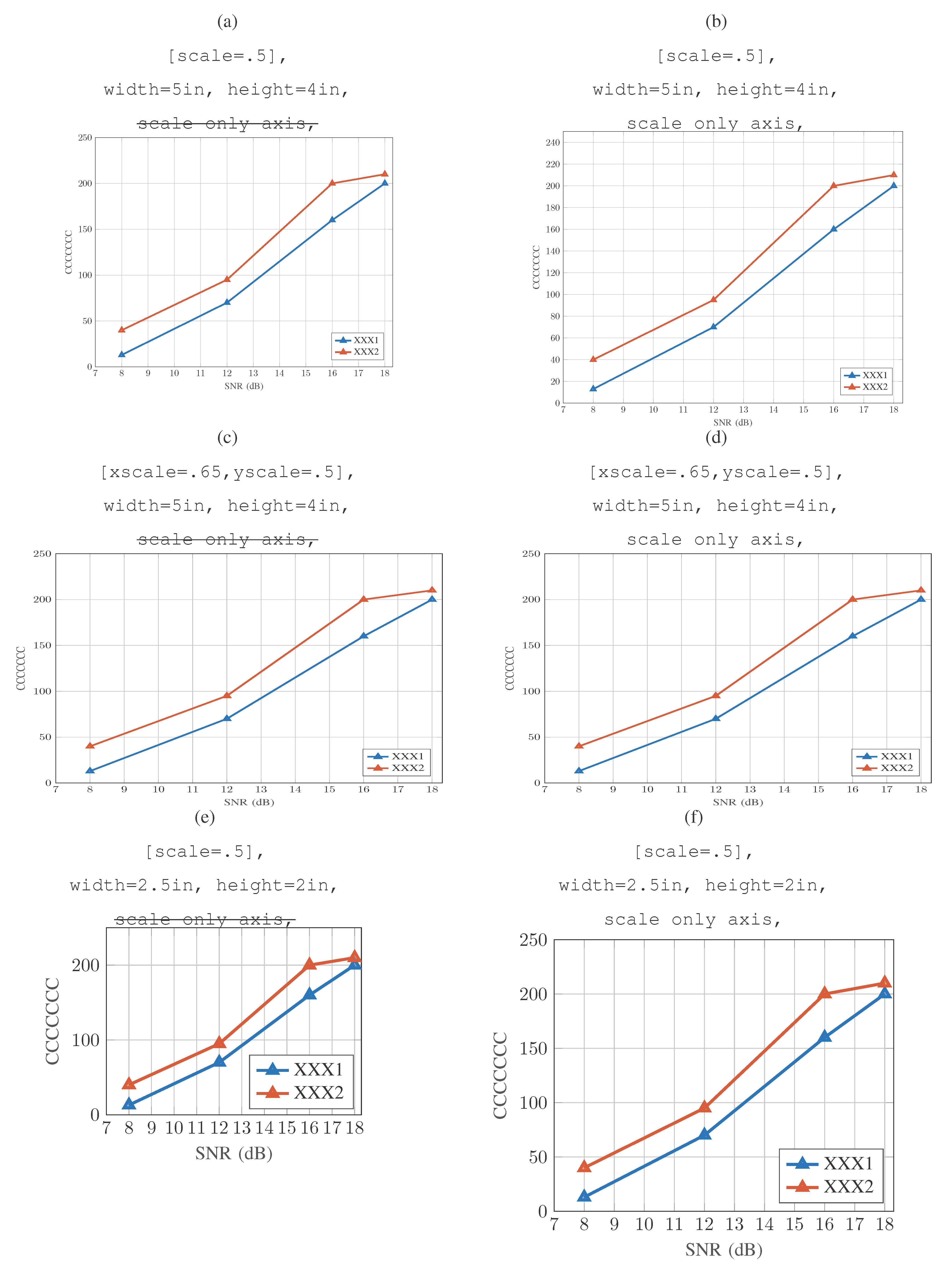
主要涉及两方面的调整：①对整个\begin{tikzpicture}环境的大小调整；②对画幅尺寸的调整（即axis环境中height和witdh的调整）

首先建议将axis环境中的at={(0.758in,0.481in)}, scale only axis,两行注释，大家一会可以尝试一下不注释这两行的效果，选择自己想要的效果。

对整个tikzpicture环境的调整：加上\begin{tikzpicture}[scale=.65]能够对整个图片的大小进行调整为原来的xx倍。
1. 同时可以使用xscale和yscale命令对横纵进行不同大小的缩放，达到拉伸的效果。
2. 注意这样的调整是对整体的调整，所有曲线、坐标、字符均进行等同的大小缩放。
axis环境中height和witdh是调整的图片原始的比例。
1. 注意这样的调整实际上是调整了原始画幅的大小，相当于在matlab中对生成的figure窗口进行拉伸缩放操作。
2. 光调整这两个参数，虽然latex中图片大小变化了，可以注意到所有曲线、坐标、字符和原始大小不变。

建议大家综合考量两个调整方式，以使得图片尺寸和字体、mark大小等均比较合适。

给出一个例子：
scale_figure

坐标轴

主要包括以下几个方面：

坐标轴的取值范围：调整xmin,xmax,ymin,ymax即可
四边坐标轴的黑边：如果想让四边均为黑色的可以把axis x line*=bottom,axis y line*=left,注释掉
增加tick：例如原来坐标轴只标注了2,4,6,8，想标注更多1,2,3,4,5,6,7，则增加一行(对y坐标轴同理)
1
xtick={1,2,3,4,5,6,7},
增加tick（光增加灰色线条，不增加标注坐标轴数字）：则增加以下三行（对y坐标轴同理）
1
2
3
extra x ticks={1,2,3,4,5,6,7,8,9},
extra x tick style={grid=major},
extra x tick labels={},
如果想要进一步挤压tick数字和label之间的距离可以加入这一行代码，但是会很紧（注意至少加在y label后面）
1
2
3
every axis y label/.style={
at={(ticklabel cs:0.5)},rotate=90,anchor=center,
},

图例

主要介绍：①位置，②字体大小，③透明度表现形式，④图例内容

matlab2tikz生成的图例相关的指令通常类似于

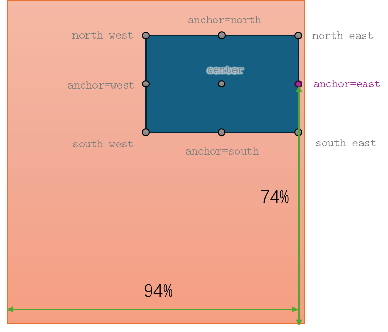
1	legend style={at={(0.97,0.74)}, anchor=east, legend cell align=left, align=left, draw=white!15!black}

首先说明以下这里面关于位置的一些说明
- at={(0.97,0.74)}指定legend框的端点在整个图片横纵坐标的比例位置，即放置在横向97%位置，纵向74%位置。
- 上面所谓的端点又是什么呢？它由anchor决定，表示端点和legend的位置关系。
调整图例的字体大小可以通过font=\scriptsize来调整。
介绍一个比较好看的legend表现形式（我们可以观察到python的legend的底框是透明的，可以透出下面的线条），如何在tikz完成呢？
- 在{}中增加以下的代码即可，
  1
  fill opacity=0.7,text opacity=1
- 这表示legend框的填充透明度为0.7（越高越不透明），文字完全不透明，大家可以适度调整
matlab2tikz的图例内容来源来源于跟在每条线条画图\addplot后面的\addlegendentry{XXX}，大家想要修改线条的图例名称直接在这里修改即可。这里支持latex的公式语法哦！

曲线相关

曲线数值的来源\addplot中的table的数值，如果想要修改/增减曲线的点，直接修改table数值即可。

曲线相关的美化主要介绍：①线条类型、粗细；②mark大小；③颜色、透明度；④线条的增删

线条类型、粗细：
- 线宽由line width=1.5pt控制，一般我觉得1.5pt-2.0pt是比较明显清晰的粗细
- 实线类型没什么好说的
- 对于虚线由matlab2tikz生成的虚线比较奇怪，我们可以将dashed修改为dash pattern=on 6pt off 3pt，这是我尝试下来比较不错的pattern。
- 还有一些其他的pattern可以参考TiKZ 线条绘制的控制 - LaTeX工作室 (latexstudio.net)
mark大小：这是我觉得matlab2tikz控制的比较不好的一点，由它生成的mark不知道为什么大大小小的，大家可以统一为mark size=3.0pt或者4.0pt左右。
颜色、透明度：
- 曲线和mark的颜色由color=mycolor1控制，大家可以自己在画图的顶上定义自己喜欢的颜色
- 如果想要让mark有填充，并且存在透明度。可以将
  - ①原始的mark均加上*，如mark=diamond*、mark=triangle*等。注意原来代表mark形状为圆圈的o直接改为*即可。
  - ②mark options={solid, mycolor2}增加fill opacity=0.5，变为mark options={solid, mycolor2, fill opacity=0.5}
线条的删除——直接将该线条对应的\addplot直到\addlegendentry删除
线条的增加——复制别的线条对应的\addplot直到\addlegendentry，修改对应的颜色、数值等

一些别的操作实例

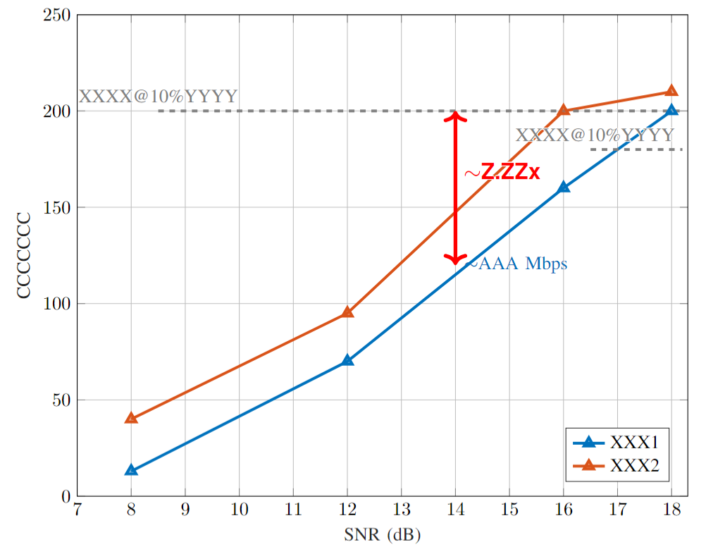
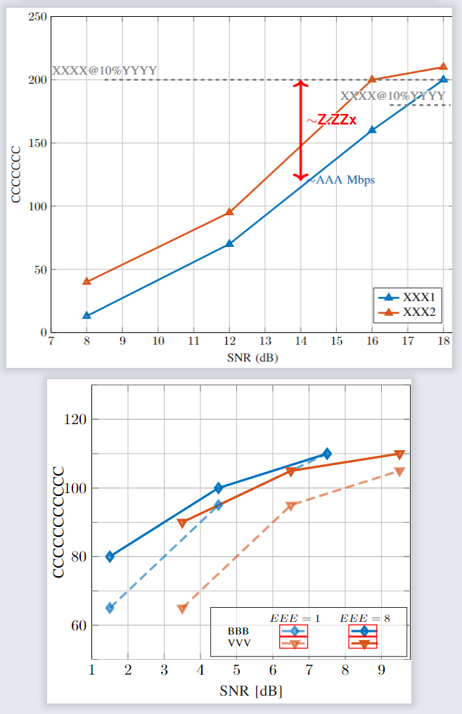
新增线条的标注——如水平线条、垂直线条

下面直接通过一个实例来解释——实例内数值均无实际含义

该实例主要包含以下几个操作

描边文字\contour{white}{$\sim$Z.ZZx}：这样主要可以使得文字可以更加明显的显示

绘制虚线并在线上标注：

1	\draw[gray, line width=1.5pt, dashed] (8.5, 200) node[ above] {\contour{white}{XXXX@10\%YYYY}}-- (18.2, 200) ;

绘制双箭头线并多个标注：

1	\draw[red, line width=2pt, <->] (14, 120)node[right]{\color{mycolor1} $\sim$AAA~Mbps} -- (14, 200) node[midway, above right, red, font=\bfseries\sffamily\large] {\contour{white}{$\sim$Z.ZZx}}

%% 以下代码会用到，请在导言区加入
% \usepackage{xcolor}
% \usepackage{contour} % 导入 contour 库，实现描边文字

%% document环境内
\definecolor{mycolor1}{rgb}{0.00000,0.44700,0.74100}%
\definecolor{mycolor2}{rgb}{0.85000,0.32500,0.09800}%
\definecolor{mycolor3}{rgb}{0.92900,0.69400,0.12500}%
\definecolor{mycolor4}{rgb}{0.49400,0.18400,0.55600}%
\definecolor{mycolor5}{rgb}{0.46600,0.67400,0.18800}%
\definecolor{mycolor6}{rgb}{0.63529,0.07843,0.18431}%
%
\begin{tikzpicture}[scale=.8]

\begin{axis}[%
width=4.521in,
height=3.566in,
at={(0.758in,0.481in)},
scale only axis,
xmin=7,
xmax=18.3,
xtick={ 7,  8,  9, 10, 11, 12, 13, 14, 15, 16, 17, 18},
xlabel style={font=\color{white!15!black}},
xlabel={SNR (dB)},
ymin=0,
ymax=250,
ylabel style={font=\color{white!15!black}},
ylabel={CCCCCCC},
axis background/.style={fill=white},
xmajorgrids,
ymajorgrids,
legend style={at={(0.97,0.03)}, anchor=south east, legend cell align=left, align=left, draw=white!15!black}
]

\addplot [color=mycolor1, line width=1.5pt, mark size=3.0pt, mark=triangle*, mark options={solid, mycolor1, fill opacity=0.5}]
  table[row sep=crcr]{%
8	13\\
12	70\\
16	160\\
18  200\\
};
\addlegendentry{XXX1}
\addplot [color=mycolor2, line width=1.5pt, mark size=3.0pt, mark=triangle*, mark options={solid, mycolor2, fill opacity=0.5}]
  table[row sep=crcr]{%
8	40\\
12	95\\
16	200\\
18  210\\
};
\addlegendentry{XXX2}

% 添加虚线
\draw[gray, line width=1.5pt, dashed] (8.5, 200) node[ above] {\contour{white}{XXXX@10\%YYYY}}-- (18.2, 200) ;

\draw[gray, line width=1.5pt, dashed] (16.5, 180) -- (18.2, 180) node[ above left] {\contour{white}{XXXX@10\%YYYY}};

% 添加箭头线
\draw[red, line width=2pt, <->] (14, 120)node[right]{\color{mycolor1} $\sim$AAA~Mbps} -- (14, 200) node[midway, above right, red, font=\bfseries\sffamily\large] {\contour{white}{$\sim$Z.ZZx}};
\end{axis}
\end{tikzpicture}%

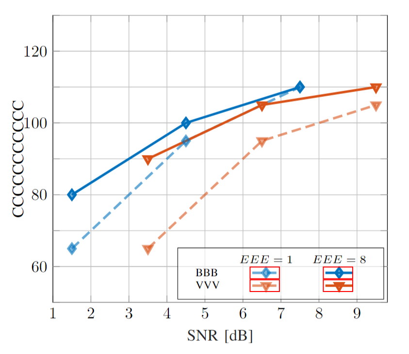
`\label`和`\ref`来构造不一般的legend

下面直接通过一个实例来解释——实例内数值均无实际含义

该实例主要包含以下几个操作

使用\label和\ref来构造不一般的legend

\definecolor{mycolor1}{rgb}{0.00000,0.44706,0.74118}%
\definecolor{mycolor3}{rgb}{0.85098,0.32549,0.09804}%
%
\begin{tikzpicture}

\begin{axis}[%
width=3.5in,
height=3.1in,
xmin=1,
xmax=9.8,
xlabel style={font=\color{white!15!black}},
xlabel={SNR [dB]},
ymin=50,
ymax=130,
ylabel style={font=\color{white!15!black}},
ylabel={CCCCCCCCCCC},
every axis y label/.style={
at={(ticklabel cs:0.5)},rotate=90,anchor=center,
},
axis background/.style={fill=white},
xmajorgrids,
ymajorgrids,
xtick={1,2,3,4,5,6,7,8,9},
extra y ticks={50,60,70,80,90,100,110,120,130},
extra y tick style={grid=major},
extra y tick labels={},
legend style={at={(0.99,0.01)}, anchor=south east, legend cell align=left, align=left, draw=white!15!black,fill opacity=0.6,text opacity=1,font=\scriptsize}
]
\addlegendimage{empty legend}
\addlegendentry[text depth=]{\begin{tabular}{lcc}
         & $EEE=1$  & $EEE=8$\\
        BBB & \protect\ref{pgf:bbb_1} & \ref{pgf:bbb_8}\\
        VVV  & \protect\ref{pgf:vvv_1}&\ref{pgf:vvv_8}\\ 
    \end{tabular}}
    
\addplot [color=mycolor1, dash pattern=on 6pt off 3pt, line width=1.5pt, mark size=3.0pt, mark=diamond*, mark options={solid, mycolor1, fill opacity=0.5}, opacity=0.6]
  table[row sep=crcr]{%
1.5	65\\
4.5	95\\
7.5	110\\
};
\label{pgf:bbb_1}
% \addlegendentry{BBB (1)}

\addplot [color=mycolor1, line width=1.5pt, mark size=3.0pt, mark=diamond*, mark options={solid, mycolor1, fill opacity=0.5}]
  table[row sep=crcr]{%
1.5	80\\
4.5	100\\
7.5	110\\
};
\label{pgf:bbb_8}
% \addlegendentry{BBB (8)}

\addplot [color=mycolor3, dash pattern=on 6pt off 3pt, line width=1.5pt, mark size=3.0pt, mark=triangle*, mark options={solid, rotate=180, mycolor3, fill opacity=0.5, fill opacity=0.5}, opacity=0.6]
  table[row sep=crcr]{%
3.5	65\\
6.5	95\\
9.5	105\\
};
\label{pgf:vvv_1}
% \addlegendentry{vvv (1)}

\addplot [color=mycolor3, line width=1.5pt, mark size=3.0pt, mark=triangle*, mark options={solid, rotate=180, mycolor3, fill opacity=0.5}]
  table[row sep=crcr]{%
3.5	90\\
6.5	105\\
9.5	110\\
};
\label{pgf:vvv_8}
% \addlegendentry{vvv (8)}

\end{axis}
\end{tikzpicture}%

将TikZ绘图保存为PDF

preview宏包

可以使用preview宏包来创建只含有tikz画图的PDF文件

1
2
3

\usepackage[active,pdftex,tightpage]{preview}
\PreviewEnvironment{tikzpicture}
\setlength{\PreviewBorder}{0.5bp}

注意\setlength{\PreviewBorder}{0.5bp}设置的是图片周围白边的宽度为0.5bp

生成结果如下

大家再采用Adobe Acrobat等工具分开每张图即可。

【附】脚本删除所有PDF文件的白边

例如用于PowerPoint/MATLAB绘图导出的PDF文档

安装texlive的时候会安装一个脚本pdfcrop，定位到需要删除白边的文件夹下在命令行中输入该代码能够将所有的PDF结尾的图片的白边全都去除。

1	for %i in (*.pdf) do pdfcrop %i %i

该博客都是一些自己的探索和方法，如果有错误、缺漏、不足，欢迎在评论区指出！

［暴论］ChatGPT就是最好的老师！

LaTeX\LaTeXLATE​X札记（六）——MATLAB与TikZ绘图