/ 实验  

电磁场实验

电磁场实验

这是电磁场实验虚拟仿真的部分内容思路,后续应该有空的时候会更新完四个实验。

实验四一开始左旋右旋判断错了,现在刚刚讲到。如果老师看到这里,能不能不算错啊🤣

——2020年6月2日

实验一 带电粒子在电磁场中的受力与运动特性研究实验

这个实验说实话像是物理实验,不是很像电磁场实验🤣。物理实验貌似真的做过这个类似的。

基础部分

编写程序,用MATLAB数值模拟的方法,模拟带电粒子在均匀分布的正交电磁场中的螺旋运动,带电粒子进入磁场的方向与磁场方向之间的夹角为θ\theta,(0<θ<90°0<\theta<90°)。

设带电粒子的初始状态如下:

粒子带电量qq=1.6×10²C,粒子质量mm=0.02g. \begin{aligned} \text{粒子带电量$q$: } &\quad q=1.6\times 10^{-2} C, \\ \text{粒子质量$m$: }&\quad m=0.02 g. \end{aligned}

根据题设,我们要模拟三种状态,分别设参数如下:

  • 电场强度和磁场强度都不为零,B=2,E=2B=2,E=2;

  • 电场强度为零,磁场强度不为零,B=2,E=0B=2,E=0;

  • 电场强度不为零,磁场强度为零,B=0,E=2B=0,E=2

利用上学期在*《计算方法》*中学到的Runge-Kutta算法即可求解该问题。

odefun1.m

1
2
3
4
5
6
7
8
function dwdt = odefun1(t,w,q,B,m,E)
dwdt = zeros(6,1);
dwdt(1) = w(2);
dwdt(2) = q.*B.*w(4)./m;
dwdt(3) = w(4);
dwdt(4) = q.*E./m-q.*B.*w(2)./m;
dwdt(5) = w(6);
dwdt(6) = 0;

针对微分方程组的初始条件y0,设初值条件w1=0w_1=0,w2=0.01w_2=0.01,w3=0w_3=0,w4=6w_4=6,w5=0w_5=0,w6=0.01w_6=0.01开始迭代,得到[t,w]的关系值。由于w1=xw_1 = xw3=yw_3 = yw5=zw_5 = z,所以我们依据不同时刻带电粒子的位置利用三维绘图函数plot3绘制图像。选择不同的ii值即可绘制三种不同情况的带电粒子运动轨迹。具体程序如下:

lab011.m

1
2
3
4
5
6
7
8
9
10
11
12
13
14
15
16
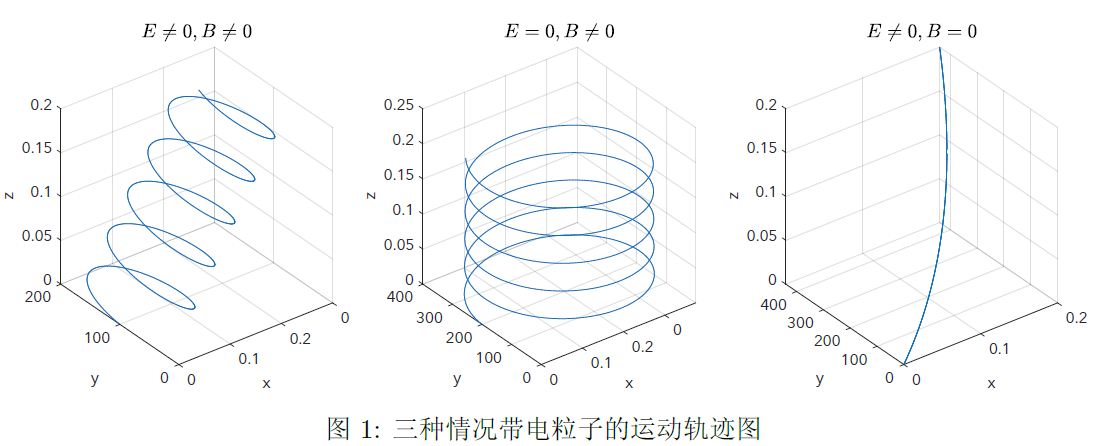
%% The movement of charged particles in an electromagnetic field (full image)
global q m B E
q=1.6e-2; % Charge of particle
m=0.02; % Mass of particle
B=[2;2;0]; % Magnetic flux density in orthogonal electromagnetic field, single magnetic field, single electric field
E=[2;0;2]; % Electric field strength under orthogonal electromagnetic field, single magnetic field, single electric field
fig{1}='$E\not= 0,B\not= 0$';
fig{2}='$E=0,B\not= 0$';
fig{3}='$E\not= 0, B=0$';
for i=1:3 % Choose a different i, switch between "orthogonal electromagnetic field", "single magnetic field", "single electric field"
[t,w]=ode23(@(t,w) odefun1(t,w,q,B(i),m,E(i)),[0:0.01:20],[0,0.01,0,6,0,0.01]);
subplot(1,3,i),plot3(w(:,1),w(:,3),w(:,5));
grid on
title(fig{i},'fontsize',12,'Interpreter','latex');
xlabel('x'); ylabel('y'); zlabel('z');
end

lab01-1

发挥部分

vv放到笛卡尔坐标系中讨论,则可得到带电粒子的位置方程

{x=v//t=vtcosθ,y=vcos(ωt)=vsinθcos(ωt),z=vsin(ωt)=vsinθsin(ωt).\left\{\begin{aligned} x&=v_{//}t=vt\cos \theta ,\\ y&=v_{\bot}\cos{(\omega t)}=v\sin \theta\cos(\omega t),\\ z&=v_{\bot}\sin{(\omega t)}=v\sin \theta\sin(\omega t). \end{aligned}\right.

为了使所有点从同一位置发射出(t=0t=0时,x=y=z=0x=y=z=0),并简单化初始参数(令v=1,ω=1v=1,\omega=1),可以将方程改写为

{x=tcosθ,y=sinθ(1+cos(tπ)),z=sinθsin(tπ).\left\{\begin{aligned} x&=t\cos \theta ,\\ y&=\sin \theta(1+\cos(t-\pi)),\\ z&=\sin \theta\sin(t-\pi). \end{aligned}\right.

θ\theta很小时,v//v,vvθv_{//}\approx v,\,v_{\bot}\approx v \theta。发散角不太大的带电粒子束,经一个周期后重新会聚。这里我们取出射角度θ[10,10]\theta\in[-10^\circ,10^\circ]

为了进一步观察每一个带电粒子束的运动轨迹,我们选用彗星图comet3函数。彗星图是动画图,其中一个圆(彗星头部)跟踪屏幕上的数据点。彗星主体是位于头部之后的尾部。尾巴是跟踪整个函数的实线。comet3(x,y,z) 显示经过点 [x(i),y(i),z(i)][x(i),y(i),z(i)] 曲线的彗星图。

lab012.m

1
2
3
4
5
6
7
8
9
10
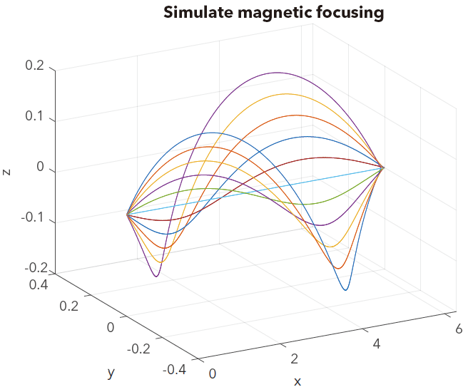
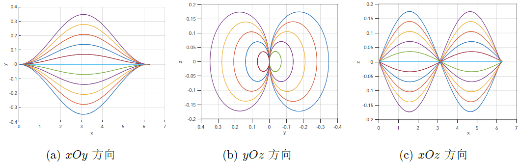
%% Simulate magnetic focusing
t=0:0.01:2*pi;
for theta=[-10:2:10]*pi/180;
grid on;
hold on;
% comet3(cos(theta).*t,sin(theta).*(cos(t-pi)+1),sin(theta).*sin(t-pi));
plot3(cos(theta).*t,sin(theta).*(cos(t-pi)+1),sin(theta).*sin(t-pi));
end
xlabel('x'); ylabel('y'); zlabel('z');
title('Simulate magnetic focusing')

lab01-2a

lab01-2b

提高部分

设带电粒子的初始状态如下:

粒子带电量qq=1.6×10¹⁹C,粒子质量mm=1.67×1027g,初速度v0v0=1×10⁶m/s,初始磁场B0B0=1T,磁场变化速率:Bzz=10T/m.\begin{aligned} \text{粒子带电量$q$:} &\quad q=1.6\times 10^{-19} C, \\ \text{粒子质量$m$:}&\quad m=1.67\times 10^{-27} g,\\ \text{初速度$v_0$:}&\quad v_0=1\times 10^6 m/s,\\ \text{初始磁场$B_0$:}&\quad B_0=1 T,\\ \text{磁场变化速率:}&\quad \frac{\partial B_z}{\partial z}=10 T/m. \end{aligned}

针对"磁镜效应",可以被转化为

{dw1dt=w2;dw2dt=qw4m(10w5+1)qw6m(5w12+w32cos(π4));dw3dt=w4;dw4dt=qw6m(5w12+w32sin(π4));dw5dt=w6;dw6dt=qw4m(5w12+w32sin(π4))\left\{\begin{aligned} \frac{\mathrm{d}w_1}{\mathrm{d}t} &= w_2;\\ \frac{\mathrm{d}w_2}{\mathrm{d}t} &= \frac{qw_4}{m}(10w_5+1)-\frac{qw_6}{m}\left(-5\sqrt{w_1^2+w_3^2}\cos\left(\frac{\pi}{4}\right)\right);\\ \frac{\mathrm{d}w_3}{\mathrm{d}t} &= w_4;\\ \frac{\mathrm{d}w_4}{\mathrm{d}t} &= \frac{qw_6}{m}\left(-5\sqrt{w_1^2+w_3^2}\sin\left(\frac{\pi}{4}\right)\right);\\ \frac{\mathrm{d}w_5}{\mathrm{d}t} &= w_6;\\ \frac{\mathrm{d}w_6}{\mathrm{d}t} &= -\frac{qw_4}{m}\left(-5\sqrt{w_1^2+w_3^2}\sin\left(\frac{\pi}{4}\right)\right) \end{aligned}\right.

odefun2.m

1
2
3
4
5
6
7
8
function dwdt = odefun2(t,w,q,m)
dwdt = zeros(6,1);
dwdt(1) = w(2);
dwdt(2) = q*(10*w(5)+1)*w(4)/m-q*((-5*sqrt(w(1).^2+w(3).^2))*cos(pi/4))*w(6)/m;
dwdt(3) = w(4);
dwdt(4) = q*((-5*sqrt(w(1).^2+w(3).^2))*sin(pi/4))*w(6)/m;
dwdt(5) = w(6);
dwdt(6) = -q*((-5*sqrt(w(1).^2+w(3).^2))*sin(pi/4))*w(4)/m

lab013.m

1
2
3
4
5
6
7
8
9
10
%% Magnetic mirror effect
q=1.6e-19; % Charge of particle
m=1.67e-27; % Mass of particle
v0=1e6; % Initial velocity
theta=pi/4; % Shooting speed
Vy=0,Vz=v0*cos(theta),Vx=v0*sin(theta);
[t,w]=ode45(@(t,w) odefun2(t,w,q,m),[0:1e-7:1.5e-6],[0,Vx,1.1,Vy,0,Vz]);
plot3(w(:,1),w(:,3),w(:,5)); %Three-dimensional trajectory of particles
xlabel('x');ylabel('y');zlabel('z');
grid on;title('Magnetic mirror effect')

lab01-3

参考文献

  1. 孙志忠,吴宏伟,袁慰平等.计算方法与实习(第5版)[M].南京:东南大学出版社,2011.
  2. 任海林.带电粒子在均匀稳定电磁场中的运动分析与编程演示[EB/OL].https://wenku.baidu.com/view/066a56ee5ef7ba0d4a733bff.html,2011-02-06/2020-04-07.
  3. 方瑞银,戚海洋.MATLAB仿真带电粒子在磁场中磁镜现象[J]. 电子世界, 2012(21):94-95.
  4. 代国红,李兴鳌,黄伟军,方利广.带电粒子在磁镜场中运动时速度的演变[J].物理与工程,2010(3):17-18,36.

实验二 静电场边值问题研究实验

这个实验说起来就比其他三个实验要平和很多

仿真设置参数

由于针对两个仿真的操作基本一致,所以仅在不同的地方加以标注。

  1. 调出pdemodeler工具箱,设置网格。

  2. 区域设置:选择工具栏的画矩形工具,确定计算范围。

  3. 应用模式:在菜单栏中单击Option下拉列表框,选择Applications,再选择Electrostatics(静电学)应用模式。

  4. 边界条件:进入Boundary Mode,再选择Specify Boundary Conditions...

    • 对于平行板电容:

      • 在左边界,选择Neumann条件,g=0g=0q=0q=0

      • 在右边界,选择Neumann条件,g=0g=0q=0q=0

      • 在上边界,选择Diriehlet条件,h=1h=1r=100r=100

      • 在下边界,选择Diriehlet条件,h=1h=1r=100r=-100

    • 对于加盖导电槽:

      • 在左边界,输入Diriehlet条件,h=1h=1r=0r=0

      • 在右边界,输入Diriehlet条件,h=1h=1r=0r=0

      • 在上边界,选择Diriehlet条件,h=1h=1r=100r=100

      • 在下边界,选择Diriehlet条件,h=1h=1r=0r=0

  5. 方程参数:在菜单栏中单击PDE按钮打开PDE Spacification对话框,设介电常数ε\varepsilon为epsilon=1=1,为体电荷密度ρ\rho为rho=0=0

  6. 图形解显示参数设置1:单击工具栏的Plot Selection(类似MATLAB线稿的一个图标)中选择Color、Height(3-D plot)、Plot in x-y grid和Show mesh四项.并在Contour plot levels中设置等位线条数,在Colormap中选择配色后,单击plot按钮,画出电位的三维曲面图。

  7. 图形解显示参数设置2:单击工具栏的Plot Selection(类似MATLAB线稿的一个图标)中选择Color、Contour和Arrows三项.并在Contour plot levels中设置等位线条数,在Colormap中选择配色后,单击plot按钮,画出电位的xyx-y方向曲线图,图上的箭头是电力线方向。

实验结果

虚拟仿真平行板电容器与加盖导体槽内的电位分布

lab02-1-3D lab02-1-xy

虚拟仿真平行板电容器与加盖导体槽内的电位分布

lab02-2-3D lab02-2-xy

参考文献

实验三 平面电磁波的反射和干涉实验

实验结果

平面电磁波向理想导体垂直入射的仿真结果

入射波垂直入射到z=0z = 0的无限大理想导电平面上,两区域的的本构参数分别取为:

z<0:ε1=1, μ1=1, σ1=0.z>0:ε2=1, μ2=1, σ2=.\begin{aligned} z<0:&\quad \varepsilon_1=1,\ \mu_1=1,\ \sigma_1=0.\\ z>0:&\quad \varepsilon_2=1,\ \mu_2=1,\ \sigma_2=\infty. \end{aligned}

lab031

取角频率ω=π2\omega=\frac{\pi}{2},则

k1=ωμ1ε1=π2, η1=μ1ε1=1k_1=\omega\sqrt{\mu_1\varepsilon_1}=\frac{\pi}{2},\ \eta_1=\sqrt{\frac{\mu_1}{\varepsilon_1}}=1

Γ=1\varGamma=-1,故

Ei0=Er0,E_{i0}=-E_{r0},

全部的入射波被反射形成反向传播的反射波,故不存在透射波。

下图中,蓝色波形为入射波,橙色波形为反射波,绿色波形为合成的驻波。蓝绿色透明平面代表无耗介与理想导体的分界面。

lab031

令入射波振幅Ei0=1E_{i0}=1。 入射波:

电场:Ei=a^xEi0ejk1z=a^xejπ2z磁场:Hi=a^y1η1Ei0ejk1z=a^yejπ2z电场随时间形式:Ei(z,t)=a^xEi0cos(ωtk1z)=a^xcos(π2tπ2z)\begin{aligned} \text{电场:}&\quad{\vec E_i}={\hat a_x}{E_{i0}}{e^{-j{k_1}z}}={\hat a_x}{e^{-j{\frac{\pi}{2}}z}}\\ \text{磁场:}&\quad{\vec H_i}={\hat a_y}\frac{1}{\eta_1}{E_{i0}}{e^{-j{k_1}z}}={\hat a_y}{e^{-j{\frac{\pi}{2}}z}}\\ \text{电场随时间形式:}&\quad{\vec E_i}(z,t)={\hat a_x}{E_{i0}}\cos(\omega t-k_1 z)={\hat a_x}\cos(\frac{\pi}{2}t-\frac{\pi}{2}z)\end{aligned}

反射波:

电场:Er=a^xEi0ejk1z=a^xejπ2z磁场:Hr=a^y1η1Ei0ejk1z=a^yejπ2z电场随时间形式:Er(z,t)=a^xEi0cos(ωt+k1z)=a^xcos(π2t+π2z)\begin{aligned} \text{电场:}&\quad {\vec E_r} =-{\hat a_x}{E_{i0}}{e^{ j{k_1}z}}=-{\hat a_x}{e^{ j{\frac{\pi}{2}}z}}\\ \text{磁场:}&\quad {\vec H_r} ={\hat a_y}\frac{1}{\eta _1}{E_{i0}}{e^{ j{k_1}z}}= {\hat a_y}{e^{ j{\frac{\pi}{2}}z}}\\ \text{电场随时间形式:}&\quad {\vec E_r}(z,t)=-{\hat a_x}{E_{i0}}\cos(\omega t+k_1 z)=-{\hat a_x}\cos(\frac{\pi}{2} t+\frac{\pi}{2}z)\end{aligned}

透射波:不存在

合成波(驻波):合成波为驻波,不发生能量传输过程,仅在两个波节间进行电场能量和磁场能的交换。

平面电磁波向理想介质垂直入射的仿真结果

入射波垂直入射到z=0z = 0的无限大理想介质平面上,两区域的的本构参数分别为:

z<0:ε1=1, μ1=1, σ1=0.z>0:ε2=4, μ2=1, σ2=0.\begin{aligned} z<0:&\quad \varepsilon_1=1,\ \mu_1=1,\ \sigma_1=0.\\ z>0:&\quad \varepsilon_2=4,\ \mu_2=1,\ \sigma_2=0.\end{aligned}

lab032

取角频率ω=π2\omega=\frac{\pi}{2},则

2k1=ωμ1ε1=π2, η1=μ1ε1=1k2=ωμ2ε2=π,η2=μ2ε2=12\begin{aligned}{2} &k_1=\omega\sqrt{\mu_1\varepsilon_1}=\frac{\pi}{2},&\ \eta_1=\sqrt{\frac{\mu_1}{\varepsilon_1}}=1\\ &k_2=\omega\sqrt{\mu_2\varepsilon_2}=\pi,&\eta_2=\sqrt{\frac{\mu_2}{\varepsilon_2}}=\frac{1}{2} \end{aligned}

Γ=Er0Ei0=13,T=Et0Ei0=23.\varGamma=\frac{E_{r0}}{E_{i0}}=-\frac{1}{3}, T=\frac{E_{t0}}{E_{i0}}=\frac{2}{3}.

Er0=13Ei0, Et0=23Ei0E_{r0}=-\frac{1}{3}E_{i0},\ E_{t0}=\frac{2}{3}E_{i0}

lab032

令入射波振幅Ei0=1E_{i0}=1。 入射波:

电场:Ei=a^xEi0ejk1z=a^xejπ2z磁场:Hi=a^y1η1Ei0ejk1z=a^yejπ2z电场随时间形式:Ei(z,t)=a^xEi0cos(ωtk1z)=a^xcos(π2tπ2z)\begin{aligned} \text{电场:}&\quad {\vec E_i} ={\hat a_x}{E_{i0}}{e^{ - j{k_1}z}}= {\hat a_x}{e^{ - j{\frac{\pi}{2}}z}}\\ \text{磁场:}&\quad {\vec H_i} ={\hat a_y}\frac{1}{\eta _1}{E_{i0}}{e^{ - j{k_1}z}}= {\hat a_y}{e^{ - j{\frac{\pi}{2}}z}}\\ \text{电场随时间形式:}&\quad {\vec E_i}(z,t)={\hat a_x}{E_{i0}}\cos(\omega t-k_1 z)={\hat a_x}\cos(\frac{\pi}{2} t-\frac{\pi}{2}z)\end{aligned}

反射波:

电场:Er=13a^xEi0ejk1z=13a^xejπ2z磁场:Hr=13a^y1η1Ei0ejk1z=13a^yejπ2z电场随时间形式:Er(z,t)=13a^xEi0cos(ωt+k1z)=13a^xcos(π2t+π2z)\begin{aligned} \text{电场:}&\quad {\vec E_r} =-\frac{1}{3}{\hat a_x}{E_{i0}}{e^{ j{k_1}z}}=-\frac{1}{3}{\hat a_x}{e^{ j{\frac{\pi}{2}}z}}\\ \text{磁场:}&\quad {\vec H_r} =\frac{1}{3}{\hat a_y}\frac{1}{\eta _1}{E_{i0}}{e^{ j{k_1}z}}=\frac{1}{3} {\hat a_y}{e^{ j{\frac{\pi}{2}}z}}\\ \text{电场随时间形式:}&\quad {\vec E_r}(z,t)=-\frac{1}{3}{\hat a_x}{E_{i0}}\cos(\omega t+k_1 z)=-\frac{1}{3}{\hat a_x}\cos(\frac{\pi}{2} t+\frac{\pi}{2}z)\end{aligned}

透射波:

电场:Et=23a^xEi0ejk2z=23a^xejπz磁场:Ht=23a^y1η2Ei0ejk2z=43a^yejπz电场随时间形式:Et(z,t)=23a^xEi0cos(ωtk2z)=23a^xcos(π2tπz)\begin{aligned} \text{电场:}&\quad {\vec E_t} =\frac{2}{3}{\hat a_x}{E_{i0}}{e^{-j{k_2}z}}=\frac{2}{3}{\hat a_x}{e^{-j{\pi}z}}\\ \text{磁场:}&\quad {\vec H_t} =\frac{2}{3}{\hat a_y}\frac{1}{\eta _2}{E_{i0}}{e^{-j{k_2}z}}=\frac{4}{3} {\hat a_y}{e^{-j{\pi}z}}\\ \text{电场随时间形式:}&\quad {\vec E_t}(z,t)=\frac{2}{3}{\hat a_x}{E_{i0}}\cos(\omega t-k_2 z)=\frac{2}{3}{\hat a_x}\cos(\frac{\pi}{2} t-\pi z)\end{aligned}

代码

lab031.m

1
2
3
4
5
6
7
8
9
10
11
12
13
14
15
16
17
18
19
20
21
22
23
24
25
26
27
28
29
30
31
32
33
34
35
36
37
38
39
40
41
42
43
44
45
46
47
48
49
50
51
52
53
54
55
56
57
58
59
60
61
62
63
64
65
66
67
68
69
70
71
72
73
74
75
76
77
78
79
80
81
82
83
84
85
86
87
88
89
90
91
92
93
94
95
96
97
98
99
100
101
102
103
104
105
106
107
108
109
110
111
112
113
114
115
116
117
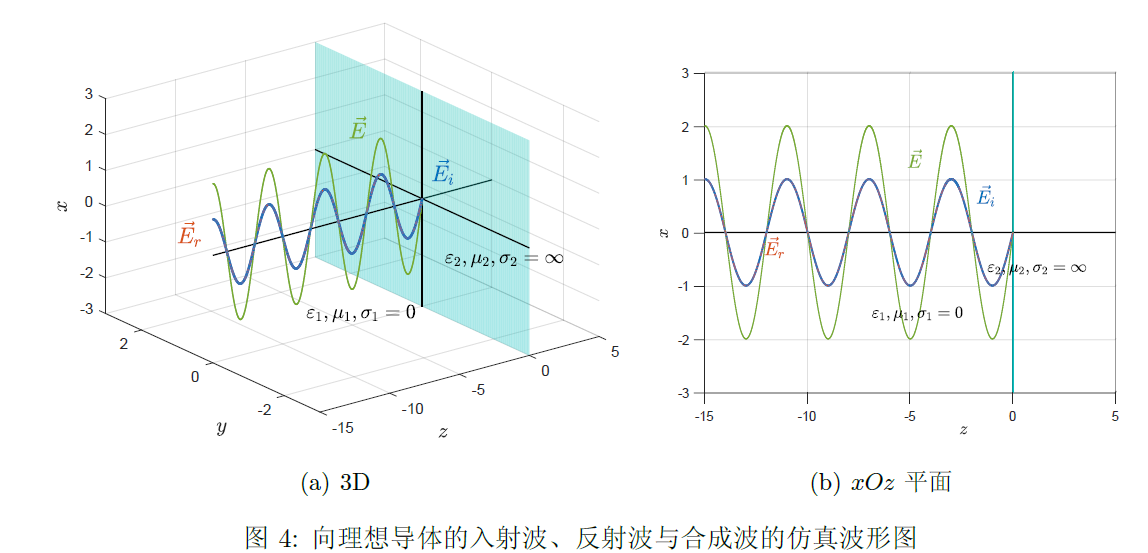
%% Perpendicular incidence to an ideal conductor
clear ,clc
E0=1; % The amplitude of the incident wave at z = 0
k1=pi/2; % phase

% Draw the interface between lossless medium and conductor
for j=1:180
display(j);
z = linspace(-3,3,100);
y = linspace(-3,3,100);
x = 0.*repmat(z,100,1) + 10000.*repmat(y,100,1);
surf(z,y,x);
alpha(.3);
shading interp
hold on
plot3 ([-15 5],[0 0],[0 0],'k','LineWidth' ,1);
hold on
plot3 ([0 0],[-3 3],[0 0],'k','LineWidth' ,1);
hold on
plot3 ([0 0],[0 0],[-3 3],'k','LineWidth' ,1);
hold on
xlabel('$z$','FontSize',14,'Interpreter','latex');ylabel('$y$','FontSize',14,'Interpreter','latex');zlabel('$x$','FontSize',14,'Interpreter','latex');
grid on
set(gca ,'XLim' ,[-15 5]);
set(gca ,'YLim',[-3 3]);
set(gca ,'ZLim',[-3 3]);
if j==1
annotation('textbox',...
[0.433214285714286 0.278523812884377 0.17979066144921 0.0733333299727666],...
'String',{'$\varepsilon_1,\mu_1,\sigma_1=0$'},...
'Interpreter','latex',...
'FontSize',13,...
'EdgeColor','none');
annotation('textbox',...
[0.651071428571428 0.393761908122476 0.195266855927426 0.0733333299727666],...
'String',{'$\varepsilon_2,\mu_2,\sigma_2=\infty$'},...
'Interpreter','latex',...
'FontSize',13,...
'EdgeColor','none');

annotation('textbox',[0.63 0.56 0.07 0.09],...
'Color',[0.00,0.45,0.74],...
'String',{'${\vec E_i}$'},...
'Interpreter','latex',...
'FontSize',15,...
'FitBoxToText','off',...
'EdgeColor','none');
annotation('textbox',[0.50 0.65 0.07 0.09],...
'Color',[0.47,0.67,0.19],...
'String','${\vec E}$',...
'Interpreter','latex',...
'FontSize',15,...
'FitBoxToText','off',...
'EdgeColor','none');
annotation('textbox',[0.23 0.43 0.07 0.09],...
'Color',[0.85,0.33,0.10],...
'String','${\vec E_r}$',...
'Interpreter','latex',...
'FontSize',15,...
'FitBoxToText','off',...
'EdgeColor','none');

% Preperation of gif
% ax = gca;
% ax.Units = 'pixels';
% pos = ax.Position;
% ti = ax.TightInset;
% rect = [-ti(1), -ti(2), pos(3)+ti(1)+ti(3), pos(4)+ti(2)+ti(4)];
% frame = getframe(ax,rect);
% im=frame2im(frame);
% k = 1;
% [I{k},map{k}]=rgb2ind(im,256);
% imwrite(I{k},map{k,1},'lab031.gif','gif','Loopcount',Inf,'DelayTime',0.1);
% k = k + 1;
end

% Preperation of drawing
z=linspace ( -15 ,0 ,1000);
y=zeros (1 ,1000);

% Electric field of incident wave
Ei=E0.*cos(-k1.*z+(j./90).*pi);
plot3(z,y,Ei ,'Color' ,[0.00,0.45,0.74],'LineWidth' ,1.5);
grid on

% Electric field of reflected wave
Er=-E0.*cos(k1.*z+(j./90).*pi);
plot3(z,y,Er ,'Color' ,[0.85,0.33,0.10],'LineWidth' ,1);

% Electric field of synthetic wave
E=E0.*cos(-k1.*z+(j./90).*pi)+E0.*cos(k1.*z+(j./180).*pi);
plot3(z,y,E,'Color' ,[0.47,0.67,0.19],'LineWidth' ,1);
M(j) = getframe;
hold off

% Get GIF
% ax = gca;
% ax.Units = 'pixels';
% pos = ax.Position;
% ti = ax.TightInset;
% rect = [-ti(1), -ti(2), pos(3)+ti(1)+ti(3), pos(4)+ti(2)+ti(4)];
% frame = getframe(ax,rect);
% im=frame2im(frame);
% [I{k},map{k}]=rgb2ind(im,256);
% imwrite(I{k},map{k},'lab031.gif','gif','WriteMode','append','DelayTime',0.1);
% k = k + 1;
end

%% Write the image to the GIF in reverse order
% for i = (k-1):-1:1
% imwrite(I{i},map{i},'lab031.gif','gif','WriteMode','append','DelayTime',0.1);
% end

%% Function to play animation
for i=1:2
movie(M,1,30);
end

lab032.m

1
2
3
4
5
6
7
8
9
10
11
12
13
14
15
16
17
18
19
20
21
22
23
24
25
26
27
28
29
30
31
32
33
34
35
36
37
38
39
40
41
42
43
44
45
46
47
48
49
50
51
52
53
54
55
56
57
58
59
60
61
62
63
64
65
66
67
68
69
70
71
72
73
74
75
76
77
78
79
80
81
82
83
84
85
86
87
88
89
90
91
92
93
94
95
96
97
98
99
100
101
102
103
104
105
106
107
108
109
110
111
112
113
114
115
116
117
118
119
120
121
%% Normal incidence to ideal medium
clear ,clc
E0=1; % The amplitude of the incident wave at z = 0
k1=pi/2;% phase
k2=pi;% phase


%% Draw the interface between lossless medium and conductor
for j=1:180
display(j);
z = linspace(-1.5,1.5,100);
y = linspace(-1.5,1.5,100);
x = 0.*repmat(z,100,1) + 10000.*repmat(y,100,1);
surf(z,y,x);
alpha(.3);
shading interp
hold on
plot3 ([-15 15],[0 0],[0 0],'k','LineWidth' ,1);
hold on
plot3 ([0 0],[-1.5 1.5],[0 0],'k','LineWidth' ,1);
hold on
plot3 ([0 0],[0 0],[-1.5 1.5],'k','LineWidth' ,1);
hold on
xlabel('$z$','FontSize',14,'Interpreter','latex');ylabel('$y$','FontSize',14,'Interpreter','latex');zlabel('$x$','FontSize',14,'Interpreter','latex');
grid on
set(gca ,'XLim' ,[-15 15]);
set(gca ,'YLim',[-1.5 1.5]);
set(gca ,'ZLim',[-1.5 1.5]);
if j==1
annotation('textbox',...
[0.433214285714286 0.278523812884377 0.17979066144921 0.0733333299727666],...
'String',{'$\varepsilon_1,\mu_1,\sigma_1=0$'},...
'Interpreter','latex',...
'FontSize',13,...
'EdgeColor','none');
annotation('textbox',...
[0.70 0.393761908122476 0.195266855927426 0.0733333299727666],...
'String',{'$\varepsilon_2,\mu_2,\sigma_2=0$'},...
'Interpreter','latex',...
'FontSize',13,...
'EdgeColor','none');

annotation('textbox',[0.45 0.65 0.07 0.09],...
'Color',[0.00,0.45,0.74],...
'String',{'${\vec E_i}$'},...
'Interpreter','latex',...
'FontSize',15,...
'FitBoxToText','off',...
'EdgeColor','none');
annotation('textbox',[0.23 0.43 0.07 0.09],...
'Color',[0.85,0.33,0.10],...
'String','${\vec E_r}$',...
'Interpreter','latex',...
'FontSize',15,...
'FitBoxToText','off',...
'EdgeColor','none');
annotation('textbox',[0.73 0.45 0.07 0.09],...
'Color',[0.47,0.67,0.19],...
'String','${\vec E_t}$',....
'Interpreter','latex',...
'FontSize',15,...
'FitBoxToText','off',...
'EdgeColor','none');

% Preperation of gif
ax = gca;
ax.Units = 'pixels';
pos = ax.Position;
ti = ax.TightInset;
rect = [-ti(1), -ti(2), pos(3)+ti(1)+ti(3), pos(4)+ti(2)+ti(4)];
frame = getframe(ax,rect);
im=frame2im(frame);
k = 1;
[I{k},map{k}]=rgb2ind(im,256);
imwrite(I{k},map{k,1},'lab032.gif','gif','Loopcount',Inf,'DelayTime',0.1);
k = k + 1;
end

% Preperation of drawing
z=linspace ( -15 ,0 ,1000);
zt=linspace (0 ,15,1000);
y=zeros (1 ,1000);

% Electric field of incident wave

Ei=E0.*cos( -k1.*z+(j./90).*pi);
plot3(z,y,Ei ,'Color' ,[0.00,0.45,0.74],'LineWidth' ,1.5);
grid on

% Electric field of reflected waves
Er=-E0.*cos(k1.*z+(j./90).*pi)./3;
plot3(z,y,Er ,'Color' ,[0.85,0.33,0.10],'LineWidth' ,1);

% Electric field of transmitted waves
Et=2*E0.*cos( -k2.*zt+(j./90).*pi)./3;;
plot3(zt ,y,Et ,'Color' ,[0.47,0.67,0.19],'LineWidth' ,1);
hold off
% N(j) = getframe;

% Get GIF
ax = gca;
ax.Units = 'pixels';
pos = ax.Position;
ti = ax.TightInset;
rect = [-ti(1), -ti(2), pos(3)+ti(1)+ti(3), pos(4)+ti(2)+ti(4)];
frame = getframe(ax,rect);
im=frame2im(frame);
[I{k},map{k}]=rgb2ind(im,256);
imwrite(I{k},map{k},'lab032.gif','gif','WriteMode','append','DelayTime',0.1);
k = k + 1;
end

%% Write the image to the GIF in reverse order
for i = (k-1):-1:1
imwrite(I{i},map{i},'lab032.gif','gif','WriteMode','append','DelayTime',0.1);
end

%% Function to play animation
% for i=1:2
% movie(N,1,30);
% end

参考文献

  1. 李丽芬,张秋菊,李扬.基于Matlab的均匀平面电磁波的仿真[J].现代电子技术,2013,36(21):136-137+140.
  2. 火星十一郎.Matlab绘制透明平面(二元函数)[EB/OL].https://www.cnblogs.com/hxsyl/p/4824884.html.2015-09-21/2020-05-11.
  3. 吕秀丽,牟海维,李贤丽.Matlab在电磁场与电磁波实验教学中之应用[J].实验室研究与探索,2010,29(02):110-112+195.
  4. 木子识时务.Matlab绘制动态 .gif 图[EB/OL].https://www.jianshu.com/p/cd9501bc810a.2017-08-20/2020-05-12.
  5. 林特斯9527.LaTeX 中插入GIF图片[EB/OL].https://www.cnblogs.com/LinTeX9527/p/11122268.html.2019-07-02/2020-05-12 .
  6. 始终.LaTeX 黑魔法(四):插入动画(animate 宏包教程)[EB/OL].https://liam.page/2017/08/10/importing-animate-in-LaTeX/.2017-08-10/2020-05-12.

主要心得

  1. MATLAB做GIF动画的感觉还是很奇妙的,以后应该会出一次博客。主要看的就是参考文献4这篇,里面的代码不用管为什么,基本上都没什么问题的,就是美中不足的是我多手八只脚(这个词多半没人听得懂),把他最后有一段反向添加进GIF的代码也贴过来了,就变成了入射波先进后出,有点怪异,但懒得在输出一次了,毕竟挺慢的。

    绘制上述两个图的程序lab031.m是一个运动的过程。其中一部份运用到了getframemoive两个函数,使动画延续多次。具体用法这里从略,有兴趣的话,可以运行程序尝试。

    另一部分用于生成GIF动图,转化后的结果如图所示。主要的函数好像是frame2imimwrite,需要先创建,后进行添加,所以这个应该有两次。

  2. 第二个“第一次”呢,就是成功在PDF文件中利用LaTeX\LaTeXanimate宏包插入了GIF(其实说不上,就只是PNG序列而已)。比较关键性的方法就是看的参考文献5、6。参考文献6很详尽的叙述了GIP转PNG图像序列的转化方式,这里用到的是一个叫ImageMagick的工具,很好用啊,但是他是命令行指令,我有点头秃。参考文献5主要侧重于LaTeX\LaTeX内部到底怎么引用怎么安排,也是拿来就能用的代码,就很好。

  3. 但是这个PDF嵌入动画效果吧,就有一个局限,该动效需要使用具备JavaScript的PDF阅读器才能观看,如Adobe Acrobat等。网上有的说福昕阅读器能开,有的说不能,还有的说很卡,我不得而知。所以我在交作业的地方留了这边的链接防止GIF放不出,也不知道老师有没有看到这里啊!

  4. 至于说实验中遇到的问题嘛,倒也不是没有,就是被一篇论文坑了。说的就是你,参考文献1!他透射波的公式Et(z,t)=23a^xEi0cos(ωtk2z)=23a^xcos(π2tπz){\vec E_t}(z,t)=\frac{2}{3}{\hat a_x}{E_{i0}}\cos(\omega t-k_2 z)=\frac{2}{3}{\hat a_x}\cos(\frac{\pi}{2} t-\pi z)k2k_2带的还是 π2\frac{\pi}{2},这就不对了啊,这个波数不是k=ωεμk=\omega\sqrt{\varepsilon\mu}嘛,k2k_2显然是k1k_1的两倍啊,所以平面电磁波向理想介质垂直入射透射波被压缩了啊。

实验四 电磁波的极化实验

实验原理

平面电磁波沿轴线前进没有 EzE_z 分量,一般情况下,存在 分量和 EyE_y 分量,如果EyE_y分量为零,只有ExE_x分量我们称其为X方向线极化。如果只有EyE_y分量而没有ExE_x分量我们称其为Y方向线极化。

在一般情况下,ExE_xEyE_y都存在,在接收此电磁波时,将得到包含水平与垂直两个分量的电磁波。如果此两个分量的电磁波的振幅和相位不同时,可以得到各种不同极化形式的电磁波。

  1. 如果电磁波场强的XXYY分量为:

Ex=Exmcos(ωt+φ1kz)Ey=Eymcos(ωt+φ2kz)\begin{aligned} {E_x}&={E_{xm}}\cos \left( \omega t+\varphi_1-kz \right)\\ {E_y}&={E_{ym}}\cos \left( \omega t+{\varphi _2}-kz \right)\end{aligned}

其中φ1\varphi_1φ2{\varphi _2}为初相位,k=2πλ\displaystyle k=\frac{2\pi }{\lambda }

φ1\varphi_1等于φ2\varphi_2,或φ1{\varphi _1}φ2\varphi_2相位差为2nπ2n\pi时,其合成电场为线极化波,其幅度为:

电场分量与XX轴的夹角为:

α=arctanEyEx=arctanEymExm=常数\alpha =\arctan \frac{E_y}{E_x}=\arctan \frac{E_{ym}}{E_{xm}}=\text{常数}

  1. 如果φ1\varphi_1φ2\varphi_2相位差90°或270°,则:

Ex=Exmcos(ωtkz+φ1)Ey=Eymcos(ωtkz+φ2)\begin{aligned} {E_x}=&{E_{xm}}\cos \left( \omega t-kz+\varphi_1 \right)\\ {E_y}=&{E_{ym}}\cos \left( \omega t-kz+\varphi_2 \right)\end{aligned}

合成电磁场为:

E=Ex2+Ey2=Exm2+Eym2=常数E=\sqrt{E_x^{2}+E_y^{2}}=\sqrt{E_{xm}^{2}+E_{ym}^{2}}=\text{常数}

它的方向是:

tanα=EyEx=tan(ωtkz+φ1)α=ωtkz+φ1\begin{gathered} \tan \alpha =\frac{E_y}{E_x}=\tan \left( \omega t-kz+\varphi_1 \right)\\ \alpha =\omega t-kz+\varphi_1\end{gathered}

表示合成场振幅不随时间变化,其方向是随时间而旋转的圆极化波。

  1. 如果其相位不为0°,180°也不是90°、270°时,合成波为椭圆极化波。

仿真程序介绍

针对电磁波的极化实验,我利用MATLAB制作了GUI界面。 如图所示,该GUI可执行程序有四部分组成:学号尾数(生成EmE_m)、仪表盘、坐标区、按钮区

电磁波的极化实验GUI界面介绍

制作GUI界面的主要步骤介绍见附录。其中三维空间中电场强度矢端轨迹为上图中右图蓝色线。图中红色带圆圈的矢量线为 z=0z=0 平面的电场强度矢量E\boldsymbol{E}。同时程序设置中设置了可以判断360°以内的极化方式,直接生成。

GUI界面主要参考台湾大学郭彦甫老师的MATLAB视频和《Matlab GUI在电磁波极化特性教学中的应用》进行设计。设计过程中主要包含两个文件:代码文件GUI4.m、图像界面文件GUI4.fig。主要过程如下:

  1. MATLABCommand Window中输入指令guide,选择Blank GUI,创建页面。
  2. 在左侧拖动控件到页面,我主要使用的是坐标区(axes), 静态文本框(Static text),可编辑文本框(Edit)。
  3. 点击绿色运行按钮(三角符号),生成GUI4.m文件,在其中编写各按键的功能。
  4. Command Window中输入指令GUI4,可运行程序。
  5. Command Window中输入指令deploytool,可打包程序为exe可执行文件,名称为Polarization_of_electromagnetic_waves.exe,文件在一般电脑上即可运行,完整的可执行exe文件看👉这里的链接。若仍有问题,具体可能需要安装MATLAB Runtime。

实验结果

设置的部分初始参数:

  • 角频率:ω=10\omega=10
  • 波数:k=π4k=\frac{\pi}{4}
  • 最大振幅:Em=5+0.1×NE_m =5+0.1\times NNN为学号尾数后两位16,即Em=6.6E_m=6.6

其他参数基本上都体现在图里了。

线极化波

- 波的传播方向:沿zz轴正方向

lab041

圆极化波

  • 波的传播方向:沿zz轴正方向

  • 圆极化旋向:顺时针,左旋圆极化波

lab042

椭圆极化波

  • 波的传播方向:沿zz轴正方向

  • 椭圆极化旋向:顺时针,左旋椭圆极化波

lab043

代码

这里只列出了其中最主要的回调函数,即按下Stimulate(仿真键)时的回调函数:

1
2
3
4
5
6
7
8
9
10
11
12
13
14
15
16
17
18
19
20
21
22
23
24
25
26
27
28
29
30
31
32
33
34
35
36
37
38
39
40
41
42
43
44
45
46
47
48
49
50
51
52
53
54
55
56
57
58
59
60
61
62
63
64
65
66
67
68
69
70
71
72
73
74
75
76
77
78
79
80
81
82
83
84
85
86
87
88
89
90
91
92
93
94
95
96
97
98
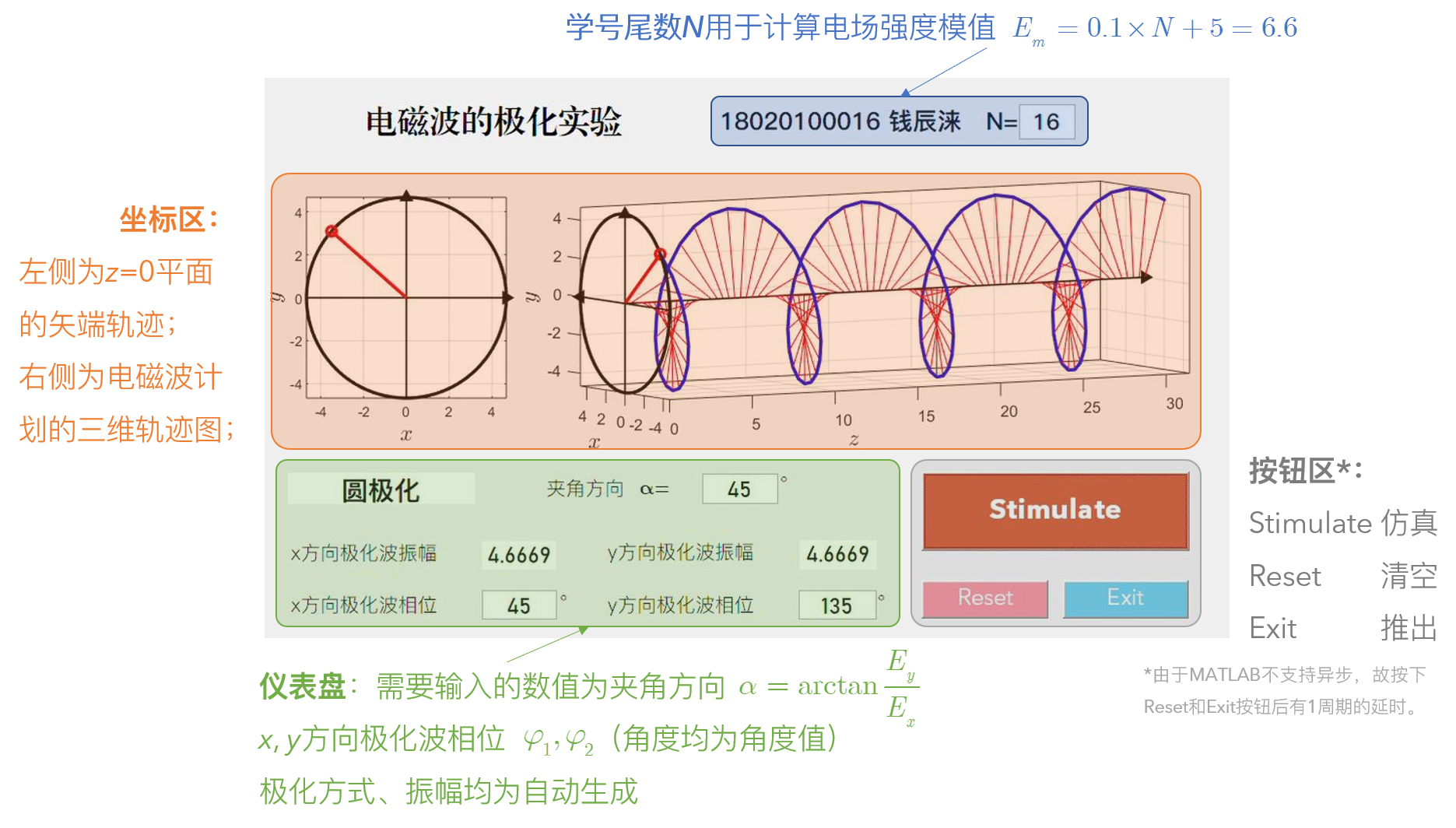
% --- Executes on button press in stimulate.
function stimulate_Callback(hObject, eventdata, handles)
% hObject handle to stimulate (see GCBO)
% eventdata reserved - to be defined in a future version of MATLAB
% handles structure with handles and user data (see GUIDATA)
clc;
% frequency and Time
omega=10;
T=2*pi/omega;
% wave speed k
k=pi/4;
% E_m: maximum of E
N=str2double(get(handles.N,'String'));
E_m=5+0.1*N;
angle=str2double(get(handles.angle,'String'));
angle_rad=angle./180.*pi;
Em_x=E_m.*cos(angle_rad);
Em_y=E_m.*sin(angle_rad);
set(handles.Em_x,'String',num2str(Em_x));
set(handles.Em_y,'String',num2str(Em_y));
E_x=[ ];E_y=[ ];
E_max=max(Em_x,Em_y);
% phi: phase
phi_x=str2double(get(handles.phi_x,'String'))*pi/180;
phi_y=str2double(get(handles.phi_y,'String'))*pi/180;
delta_phi=phi_y-phi_x;
if (mod(delta_phi,pi)==0)
set(handles.yanshi,'string','线极化');
elseif (mod(delta_phi,2*pi)==3*pi/2)
set(handles.yanshi,'string','右旋圆极化');
elseif (mod(delta_phi,2*pi)==pi/2)
set(handles.yanshi,'string','左旋圆极化');
elseif(delta_phi<0)
set(handles.yanshi,'string','右旋椭圆极化');
else
set(handles.yanshi,'string','左旋椭圆极化');
end
% other intinal settings
zmin=0;
zmax=10.*pi; % Range of z coordinate
z=zmin:pi/9:zmax;
n=length(z);

% Calculation of drawing the outline of z = 0 plane
for t1=0:0.01*T:1*T
Ex=Em_x*cos(omega*t1-k.*z+phi_x);
Ey=Em_y*cos(omega*t1-k.*z+phi_y);
E_x=[E_x Ex(1)];E_y=[E_y Ey(1)];
end
z1=zeros(length(E_x));

% Calculation of drawing dynamic simulation diagram
for t=0:0.01*T:1*T
% Calculate the magnitude of the x and y components of the electric field strength at each point
Ex=Em_x*cos(omega*t-k.*z+phi_x);
Ey=Em_y*cos(omega*t-k.*z+phi_y);

%Plot the contour of the z = 0 plane and the electric field vector at time t
axes(handles.axes1);cla(handles.axes1);
plot(E_x,E_y,'k-','LineWidth',2);
plot(Ex(1),Ey(1),'ro','LineWidth',2);
plot ([-Em_x Em_x],[0 0],'k','LineWidth' ,1);
plot (Em_x,0,'k>','LineWidth' ,1,'MarkerFaceColor','k');
plot ([0 0],[-Em_y Em_y],'k','LineWidth' ,1);
plot (0,Em_y,'k^','LineWidth' ,1,'MarkerFaceColor','k');
line([0 Ex(1)],[0 Ey(1)],'Color','r','LineWidth',2);
xlabel('$x$','FontSize',14,'Interpreter','latex');
ylabel('$y$','FontSize',14,'Interpreter','latex');
grid on;
axis equal;
axis([-Em_x,Em_x,-Em_y,Em_y]);
hold on

% Plot the outline of the z = 0 plane and the three-dimensional map of the electric field vector at time t and the dynamic map of the electric field propagation
axes(handles.axes2);cla(handles.axes2);
plot3(z1,E_x,E_y,'k-','LineWidth',2);
plot3(z,Ex,Ey,'b.-','LineWidth',2);
line([0 0],[0 Ex(1)],[0 Ey(1)],'Color','r','LineWidth',2);
plot3(z(1),Ex(1),Ey(1),'ro','LineWidth',2);
plot3 ([zmin zmax],[0 0],[0 0],'k','LineWidth' ,1);
plot3 (zmax,0,0,'k>','LineWidth' ,1,'MarkerFaceColor','k');
plot3 ([0 0],[-E_max E_max],[0 0],'k','LineWidth' ,1);
plot3 (0,E_max,0,'k<','LineWidth' ,1,'MarkerFaceColor','k');
plot3 ([0 0],[0 0],[-E_max E_max],'k','LineWidth' ,1);
plot3 (0,0,E_max,'k^','LineWidth' ,1,'MarkerFaceColor','k');
for m=1:1:n
line([z(m) z(m)],[0 Ex(m)],[0 Ey(m)],'Color','r','LineWidth',0.5);
end
grid on;
box on;
axis([zmin,zmax,-E_max,E_max,-E_max,E_max]);
axis equal;
xlabel('$z$','FontSize',14,'Interpreter','latex');
ylabel('$x$','FontSize',14,'Interpreter','latex');
zlabel('$y$','FontSize',14,'Interpreter','latex');
view(-30,5);
hold on
end

具体的代码等5月20号电磁场实验结束以后再放。

参考文献

  1. bilibili.MATLAB教程_台大郭彦甫(14课)原视频补档[V/OL].https://www.bilibili.com/video/BV1GJ41137UH?t=3177&p=7.2019-09-19/2020-05-16.
  2. 余建立.Matlab GUI在电磁波极化特性教学中的应用[J].科技创新导报,2018,15(16):244-246.

主要心得

  1. GUI界面初步入门(后续或许会写一篇博客吧)
  2. MATLAB中的GUI不支持异步,所以按下按钮差不多要等一个周期走完才行。中途试过全局变量,但是还是不行啊,如果有知道怎么异步的一定告诉我!
  3. 一开始想的是通过确定的EmE_m和待定的EmxE_{mx}来控制即可,但发现这样不可能调出正圆来(6.6太坑爹了),就只好用α=arctanEyEx\alpha=\arctan\frac{E_y}{E_x}咯!
  4. 坐标轴的一个不错的画法,再也不用annotation去凑了,其中坐标轴的箭头其实是用的数据标记的左右上下小三角实现的。
1
2
3
4
5
6
plot3 ([zmin zmax],[0 0],[0 0],'k','LineWidth' ,1);
plot3 (zmax,0,0,'k>','LineWidth' ,1,'MarkerFaceColor','k');
plot3 ([0 0],[-E_max E_max],[0 0],'k','LineWidth' ,1);
plot3 (0,E_max,0,'k<','LineWidth' ,1,'MarkerFaceColor','k');
plot3 ([0 0],[0 0],[-E_max E_max],'k','LineWidth' ,1);
plot3 (0,0,E_max,'k^','LineWidth' ,1,'MarkerFaceColor','k');
  1. 关闭Exit按钮的代码其实就一句close,清空坐标区和字符串的代码也很简单
1
2
3
4
5
6
7
% 重置清空图片 
cla(handles.axes1,'reset');
cla(handles.axes2,'reset');
% 重置清空动态txt的文字
set(handles.yanshi,'string','演示')
set(handles.angle,'string','')
set(handles.Em_x,'string','')
  1. 这次是GUI,所以不是MATLAB自动导出的GIF,而是将GUI界面的exe可执行程序运行过程录屏后,通过Premiere转换为PNG图片序列(但为什么Premiere导出来的图这么大呢,还不清楚,100K的图还不如上次实验直出的20K的图得质量好)。

本文标题:电磁场实验

文章作者:Levitate_

发布时间:2020年05月12日 - 14:21:46

原始链接:https://levitate-qian.github.io/2020/05/12/%E7%94%B5%E7%A3%81%E5%9C%BA%E5%AE%9E%E9%AA%8C/

许可协议: 署名-非商业性使用-禁止演绎 4.0 国际 转载请保留原文链接及作者。